Chapter 01 Foundations & History 1830s · Babbage → 1936 · Turing → 1948 · Shannon Where the field came from. The dreams of Babbage and Lovelace, the rigor of Hilbert, the cut of Turing, the channel of Shannon. Read this once and the rest of the curriculum maps to a place.

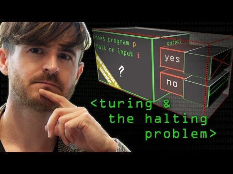

Turing machine
An imagined device with an infinite tape and a tiny rulebook. At each step it reads the symbol under its head, looks up the rule for that symbol in its current state, writes a new symbol, moves left or right, and changes state. Anything any computer can compute, a Turing machine can compute.
Alan Turing proposed this model in 1936 in 'On Computable Numbers, with an Application to the Entscheidungsproblem' to formalize what 'computable' means and to prove the Halting Problem undecidable. The Entscheidungsproblem was Hilbert's challenge: is there a mechanical procedure that decides every mathematical statement? Turing's answer: no.
A diligent clerk with an infinite scroll, a one-symbol stamp, and a flip-card of rules. The clerk has no memory of what came before this step — every decision is made from the current state and the symbol they're staring at.
A two-state Turing machine can recognize the language { 0^n 1^n | n ≥ 1 }: zero out each 0 and the matching 1 alternately, walking the tape back and forth.
# A 5-state Turing machine that accepts 0^n 1^n
def step(tape, head, state, delta):
    sym = tape[head]
    new_state, new_sym, move = delta[(state, sym)]
    tape[head] = new_sym
    head += 1 if move == "R" else -1
    return tape, head, new_state
data Move = L | R
type Delta = (State, Sym) -> (State, Sym, Move)
step :: Delta -> Tape -> Int -> State -> (Tape, Int, State)
step delta tape head state =
let (s', sym', mv) = delta (state, tape !! head)
tape' = update head sym' tape
head' = if mv == R then head + 1 else head - 1
in (tape', head', s')Church–Turing thesis

Every function that is effectively computable by any method — lambda calculus, recursive functions, Turing machines, your laptop, a quantum computer — is computable by a Turing machine. It is a thesis, not a theorem: it claims that our intuitive notion of 'effectively computable' coincides with a specific formal definition.
Alonzo Church developed the lambda calculus in 1932-1936 to formalize functions. Turing developed his machines independently in 1936. Stephen Kleene proved the two models compute the same class of functions. Church and Turing each proposed their model captured 'effective calculability'; together they form the thesis.
Different ways to describe a recipe — pictogram, English prose, a chef's flow chart — all reduce to the same dishes. Different models of computation all reduce to the same set of computable functions.
JavaScript, x86 assembly, Lisp, Conway's Game of Life, the lambda calculus, and a Turing machine are all Turing-complete — each can simulate the others. Their computable sets are identical.
Lambda calculus
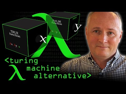

A tiny programming language with just three pieces: a variable, a function (lambda x. body), and an application (function argument). With those three you can express every computable function. Numbers, booleans, lists, recursion — all encoded as functions.
Alonzo Church, 1932-1936. He wanted a foundation for math that didn't depend on set theory. Russell's paradox had broken Frege's set theory; Church's calculus avoided self-reference by carefully distinguishing functions from their arguments. Type theory grew out of this, eventually giving us ML, Haskell, and modern type systems.
A vending machine. Insert an argument, the machine substitutes it into a slot, hands you the result. Stack vending machines and you can compute anything.
Church-encoded booleans: TRUE = λx.λy.x, FALSE = λx.λy.y. AND = λp.λq.p q p. NOT = λp.λx.λy.p y x. Numbers: 0 = λf.λx.x, 1 = λf.λx.f x, 2 = λf.λx.f (f x). Successor: SUCC = λn.λf.λx.f (n f x).
-- Identity, application, composition
id' = \x -> x
apply f x = f x
compose f g = \x -> f (g x)
-- Church numerals
zero  = \f x -> x
one   = \f x -> f x
succ' = \n f x -> f (n f x)
# Lambda calculus is a one-liner in Python
TRUE = lambda x: lambda y: x
FALSE = lambda x: lambda y: y
AND = lambda p: lambda q: p(q)(p)
# Church numerals
ZERO = lambda f: lambda x: x
SUCC = lambda n: lambda f: lambda x: f(n(f)(x))
def to_int(n): return n(lambda x: x + 1)(0)Information & entropy


Information measures surprise. A coin flip carries 1 bit because two outcomes are equally likely. A six-sided die carries log₂(6) ≈ 2.58 bits. Shannon entropy is the average surprise of a probability distribution — the lower bound on how few bits per symbol you need to encode it.
Claude Shannon, 1948, 'A Mathematical Theory of Communication' in Bell System Technical Journal. He single-handedly created the field of information theory. The paper introduced bits, entropy, channel capacity, and the noisy-channel coding theorem. Every modern modem, codec, and compression algorithm traces to it.
How many yes/no questions you need to ask to pin down a random outcome on average. Two equiprobable options: 1 question. Eight equiprobable options: 3 questions. Skewed distribution: fewer, because guessing the common one first wins.
English text averages about 1.0–1.5 bits per character even though there are 27 possible symbols (log₂(27) ≈ 4.75). Compression algorithms exploit that gap.
Chapter 02 Mathematical Foundations 1850s · Boole → 1879 · Frege → 1931 · Gödel The math your code stands on. Sets, logic, proof, induction, combinatorics, graphs, probability. Skip nothing — these are the load-bearing axioms.


Sets, relations, functions
A set is an unordered collection of distinct elements. A relation between two sets is a subset of their Cartesian product. A function is a relation where every input maps to exactly one output. From these three you build every data structure in computing.
Georg Cantor founded modern set theory in the 1870s. Russell's paradox (1901) broke naive set theory — 'the set of all sets that don't contain themselves.' Zermelo and Fraenkel patched it with axiomatic set theory (ZFC, 1908-1922), the foundation most working mathematicians use today.
A set is a sack with no order and no duplicates. A function is a no-cheating lookup table: every key has exactly one value.
Database keys form a set. A foreign-key constraint is a function from one table's rows to another's primary keys. SQL's GROUP BY partitions rows into an equivalence relation.
Mathematical induction

Prove a property P holds for every natural number by showing two things: P(0) is true, and if P(n) is true then P(n+1) is true. The dominos all fall. Strong induction lets you assume P(k) for every k ≤ n.
Pascal, Fermat, and others used induction informally in the 17th century. Peano's axioms (1889) made it rigorous. It's the workhorse proof technique for algorithms — almost every correctness proof of a recursive algorithm is induction on input size.
A domino chain. Knock over the first, and prove each domino knocks the next, and the whole chain falls.
Prove 1 + 2 + ... + n = n(n+1)/2. Base: n=1 gives 1 = 1·2/2 ✓. Step: assume true for n, then 1 + ... + (n+1) = n(n+1)/2 + (n+1) = (n+1)(n+2)/2. ✓
Chapter 03 Computability & Theory of Computation 1936 · Turing → 1956 · Chomsky → 1971 · Cook What can be computed, what cannot, and what costs how much. Finite automata, pushdown automata, Turing machines, the Chomsky hierarchy, decidability, the halting problem.

Deterministic finite automaton (DFA)

A machine with a finite set of states and a transition table. Read one input symbol, jump to the state the table says, repeat. Accept if you end in an accepting state. DFAs recognize exactly the regular languages — same expressive power as regular expressions.
Kleene's theorem (1956) proved DFAs, NFAs, and regular expressions all recognize the same languages. The Chomsky hierarchy (1956) placed regular languages at the bottom of a four-tier ladder of formal-language complexity.
A vending machine. Press a coin button — state changes. Press another — state changes again. Reach the 'dispense' state and you get a soda; reach 'invalid combo' and you get nothing.
Match the language of strings over {0,1} that contain '101'. Three states: 'haven't started', 'saw 1', 'saw 10', 'saw 101' (accept). On each input symbol the state machine advances.
The Halting problem

There is no algorithm that takes a program P and an input I and decides whether P halts on I. Not 'we haven't found one' — proven impossible. Turing's proof: assume HALT exists, build a program that asks HALT about itself and does the opposite — contradiction.
Turing, 1936, in the same paper that defined the Turing machine. The proof is the prototype for every undecidability result that followed: Rice's theorem, the Post correspondence problem, the word problem for groups.
A perfect lie detector that turns itself on. If a perfect lie detector exists, ask it 'will you say no?' — and both answers are contradictions. The Halting problem is the lie detector for 'does this program halt?'
while True: pass — clearly doesn't halt. print('hi') — clearly halts. But: while not is_perfect(n): n += 1 where is_perfect tests if n equals the sum of its proper divisors — does this halt? Open problem.
NP-completeness
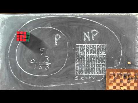
P is the class of decision problems solvable in polynomial time. NP is the class where a 'yes' answer can be verified in polynomial time given a witness. An NP-complete problem is in NP AND every other NP problem reduces to it in polynomial time. If any one NP-complete problem has a polynomial-time algorithm, P = NP.
Cook (1971) proved SAT is NP-complete — the foundational result. Karp (1972) showed 21 classical problems reduce to SAT, exploding the NP-complete class. The P vs NP question is one of the Clay Millennium Prize Problems; whoever resolves it wins $1M.
P = problems where you can quickly find an answer. NP = problems where you can quickly check an answer if someone hands you one. P = NP would mean checking is as easy as finding, which most computer scientists doubt.
3-SAT, the traveling salesman decision version, vertex cover, subset sum, graph coloring, Sudoku, and Tetris are all NP-complete. Cracking any one of them in polynomial time cracks them all.
Chapter 04 Algorithms & Complexity 1950s · Hoare → today Sorting, searching, divide-and-conquer, dynamic programming, greedy, graph algorithms. Big-O is the price tag on every algorithm.

Big-O notation

An asymptotic upper bound on a function's growth. f(n) = O(g(n)) if there are constants c, n₀ such that f(n) ≤ c·g(n) for all n ≥ n₀.
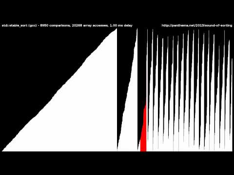
Merge sort

Recursively split the array in half, sort each half, merge them. O(n log n) worst case, O(n) extra space, stable.
Dynamic programming
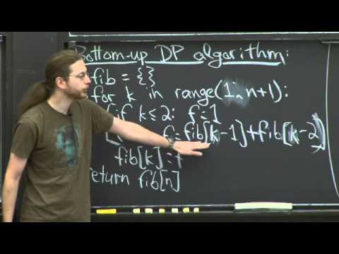
Solve a problem by combining solutions to overlapping subproblems. Memoize: cache subproblem results so each is computed once.
Chapter 05 Data Structures 1960s · Knuth → today Arrays, lists, trees, BSTs, heaps, hash tables, tries, B-trees, graphs, skip lists, persistent data structures.

Hash table
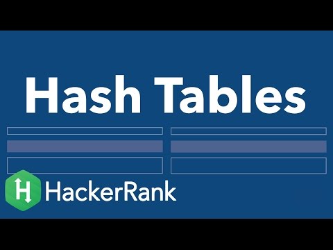
An array indexed by hash(key). Average O(1) lookup, insert, delete. Worst case O(n) when many keys collide.
B-tree
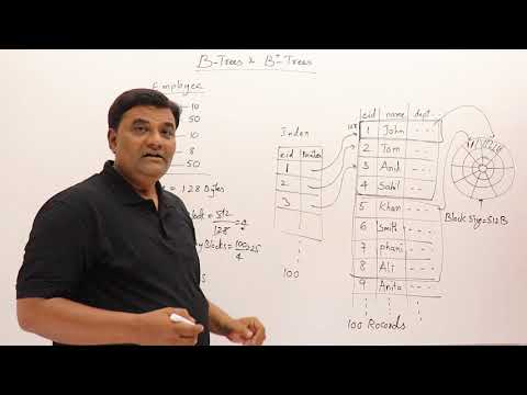
A self-balancing tree where each node holds many keys and many children. Designed for disk/SSD where reading a block is the dominant cost. Postgres, MySQL, and SQLite all use B-tree variants for indexes.
Chapter 06 Computer Architecture 1945 · von Neumann → today Logic gates, ALUs, CPU pipelines, cache hierarchies, memory, I/O, RISC vs CISC, branch prediction, speculative execution.


Von Neumann architecture
Code and data live in the same memory; a single bus moves both to the CPU. Almost every computer you've ever touched is von Neumann.
Cache hierarchy

L1 (per-core, ~1ns), L2 (per-core, ~5ns), L3 (shared, ~15ns), DRAM (~100ns), SSD (~100μs), disk (~10ms). Each level is 10–100x slower and 10–100x bigger than the one above.
Chapter 07 Operating Systems 1965 · Multics → today Processes, threads, scheduling, virtual memory, file systems, concurrency, synchronization, syscalls.
Process vs thread

A process is an isolated address space — its own memory map, file descriptors, signals. A thread is an execution context inside a process; threads in the same process share memory.
Virtual memory

Each process sees its own contiguous address space; the MMU maps virtual pages to physical frames via page tables. Pages can be swapped to disk on demand.
Chapter 08 Networks 1969 · ARPANET → today OSI/TCP-IP layers, routing, congestion control, DNS, HTTP, TLS, BGP, the actual Internet.

TCP/IP

Four layers: link (Ethernet/WiFi), network (IP — routing across networks), transport (TCP for reliable, UDP for fast), application (HTTP, DNS, SSH). Each layer wraps the one above.
TLS 1.3

Transport-layer security. Modern TLS does a Diffie-Hellman key exchange to derive a shared secret, authenticates the server via certificate signature, then encrypts the rest of the conversation with AES-GCM or ChaCha20-Poly1305.
Chapter 09 Databases 1970 · Codd → today Relational model, SQL, normalization, indexes, transactions, ACID, NoSQL, distributed databases.


ACID transactions

Atomicity (all-or-nothing), Consistency (DB invariants hold before and after), Isolation (concurrent txns don't see each other's partial work), Durability (committed data survives crashes).
Indexes
A separate data structure (usually a B-tree) that maps column values to row pointers, so range queries don't have to scan the whole table.
Chapter 10 Programming Languages 1958 · Lisp → today Type systems, parsers, semantics, paradigms: imperative, functional, logic, OO. Where languages come from and how they differ.


Type system

A set of rules that assigns each expression a type, used to prove (statically or at runtime) that the program won't go wrong. Hindley-Milner inferred types automatically; dependent types let types depend on values.
Chapter 11 Compilers 1957 · FORTRAN → today Lexing, parsing, AST, type checking, IR, optimization, codegen, register allocation.


Parsers

A parser takes a stream of tokens and builds a syntax tree according to a grammar. LL(k) parsers look k tokens ahead; LR parsers use a stack and a state table; PEG parsers express grammar as recursive descent with ordered choice.
Chapter 12 Software Engineering 1968 · NATO conference → today Testing, code review, version control, CI/CD, observability, design patterns. The craft of shipping code that doesn't fall over.

Git internals

Git is a content-addressed object store. Every blob, tree, commit, and tag is identified by the SHA-1 (or SHA-256) of its content. Branches are just pointers to commits.
Chapter 13 Artificial Intelligence & ML 1956 · Dartmouth → today Search, planning, neural networks, RL, NLP, computer vision, transformers, RLHF. The discipline that's eating computer science.
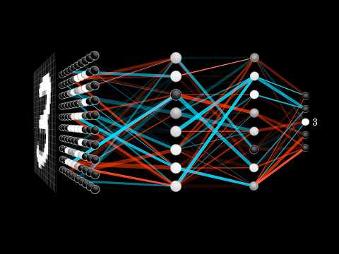
Backpropagation
The chain rule applied to a computational graph. Compute the gradient of the loss with respect to each parameter by walking the graph backwards from the output to the inputs.
Attention

An attention head computes a weighted average over a set of values, where the weights come from a similarity (softmax of QK^T) between the query and each key. Stacking many heads is what makes a Transformer.
Chapter 14 Cryptography 1976 · Diffie–Hellman → today Symmetric, asymmetric, hashing, PKI, zero-knowledge proofs, post-quantum.

Diffie–Hellman key exchange

Two parties pick private numbers a and b. Each sends g^a mod p and g^b mod p over the wire. Each can compute g^(ab) mod p, but nobody listening can — that's their shared secret.
Chapter 15 Distributed Systems 1978 · Lamport → today CAP, consensus, Paxos, Raft, gossip, replicated state machines, distributed transactions.

CAP theorem

In a partition, you must choose: consistency (every read sees the latest write) or availability (every request gets a response). You cannot have both during a network partition.
Raft consensus

An understandable consensus algorithm. A cluster elects one leader; the leader appends every command to its log and replicates to followers. A majority quorum commits each entry.
Chapter 16 Quantum Computing 1981 · Feynman → today Qubits, gates, superposition, entanglement, Shor's algorithm, Grover's algorithm, error correction.
Qubit & superposition

A qubit is a unit vector in ℂ². Measured in the {|0⟩, |1⟩} basis it collapses to 0 with probability |α|² or 1 with probability |β|². Until measurement, it's both.
Chapter 17 Formal Methods 1969 · Hoare → today Hoare logic, model checking, type theory, theorem provers (Coq, Lean, Isabelle).

Hoare logic

Reason about programs with triples {P} C {Q}: if P holds before executing C, then Q holds after — provided C terminates. The basis of every program verifier from Frama-C to Dafny to F*.
Chapter 18 Computational Geometry 1975 · Shamos → today Convex hulls, Voronoi diagrams, range trees, BSPs, computational topology.

Convex hull

The smallest convex polygon containing a set of points. Graham scan: sort by angle, walk around, pop on right turns. O(n log n).
Chapter 19 Approximation & Randomized Algorithms 1979 · Karp → today PTAS, FPTAS, Las Vegas, Monte Carlo, randomized rounding, MCMC.

Monte Carlo algorithms

A randomized algorithm with bounded runtime and bounded probability of error. Miller-Rabin primality is the textbook example: O(k) tests, error ≤ 4^-k.
Chapter 20 Research Methodology Now Reading papers, writing proofs, finding open problems, navigating a PhD. The meta-skill that turns the previous 19 chapters into research output.

Reading a CS paper
Three passes: skim (read title, abstract, intro, section headers, conclusion), reread (figures, theorems, results), and rebuild (try to derive the proofs yourself, find a hole, propose a follow-up).